VLOOKUP is undoubtedly one of the most potent tools for vertically looking up a specific keyword in a sheet. Hence, it is used in several situations to streamline workflow in countless workbooks. A similar function, HLOOKUP, is used for a horizontal lookup.
None of these lookup tools is devoid of limitations. That said, XLOOKUP is a relatively recent tool for looking up values that not only overcomes limitations but is also flexible. So, what is XLOOKUP? How can you use it in your everyday workbooks? Let’s find out.
So, without further delay, let’s start with the XLOOKUP tool on Microsoft Excel.
Format for XLOOKUP
The format for the XLOOKUP function is as follows:
=XLOOKUP(lookup_value, lookup_array, return_array, [if_not_found], [match_mode], [search_mode])
I will talk about each of the arguments now.
Looup_value (required): This is self-explanatory. It denotes the value that needs to be searched in the records. You have to enter this manually.
Lookup_array (required): The value you enter will be searched in the array. Just select the row or column where the lookup_value is supposed to exist.
Return_array (required): If a match is found, the value in this array for the matching record will be returned.
If_not_found (optional): You can display a custom error message if a match is not found.
Match_mode (optional): You must select the match type by entering four values between 0, -1, 1, and 2.
0: It looks for an exact match. If it is not found, it will display your chosen error message.
-1: If an exact match is not found, it will return the immediate smaller value based on the search.
1: If an exact match is not found, it will return the immediate larger considerable value based on the search.
2: You can use this for wildcard matches, and ‘?’,’*,’ and ‘~’ have different functions.
- Question mark (?): It looks for any character where it is entered. For example, if you enter Ro?y, it will search for Rony, Roxy, Romy, etc.
- Asterisk (*): It will search for everything, no matter the length entered. For example, if you enter south*, it will search for southeast and southwest or any other result with south at the beginning.
- Tilde (~) refers to question marks, asterisk, and tilde.
Search_mode (optional): You can select among four different search modes: 1, -1, 2, and -2.
1: It starts the search with the first item. If you don’t enter any search mode, this is the default.
-1: It starts the search with the last item.
2: It starts a binary search, where the array needs to be sorted in ascending order.
-2: It starts a binary search, where the array needs to be sorted in descending order.
*In both 2 and -2, if the array isn’t sorted as required, you will get invalid results.
With the above explanation, you can already know how powerful XLOOKUP is compared to VLOOKUP.
Explanation with an example
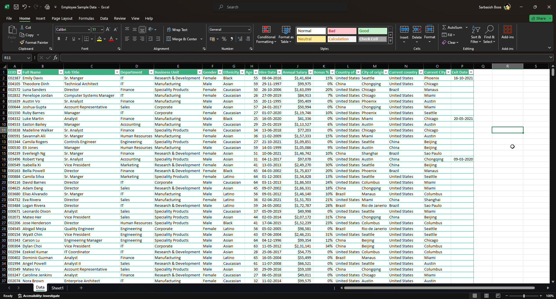
Now, let’s examine a dataset to help you better understand the XLOOKUP functions on Excel.
The dataset here includes data regarding some employees in a company, including employee ID, name, department, etc.

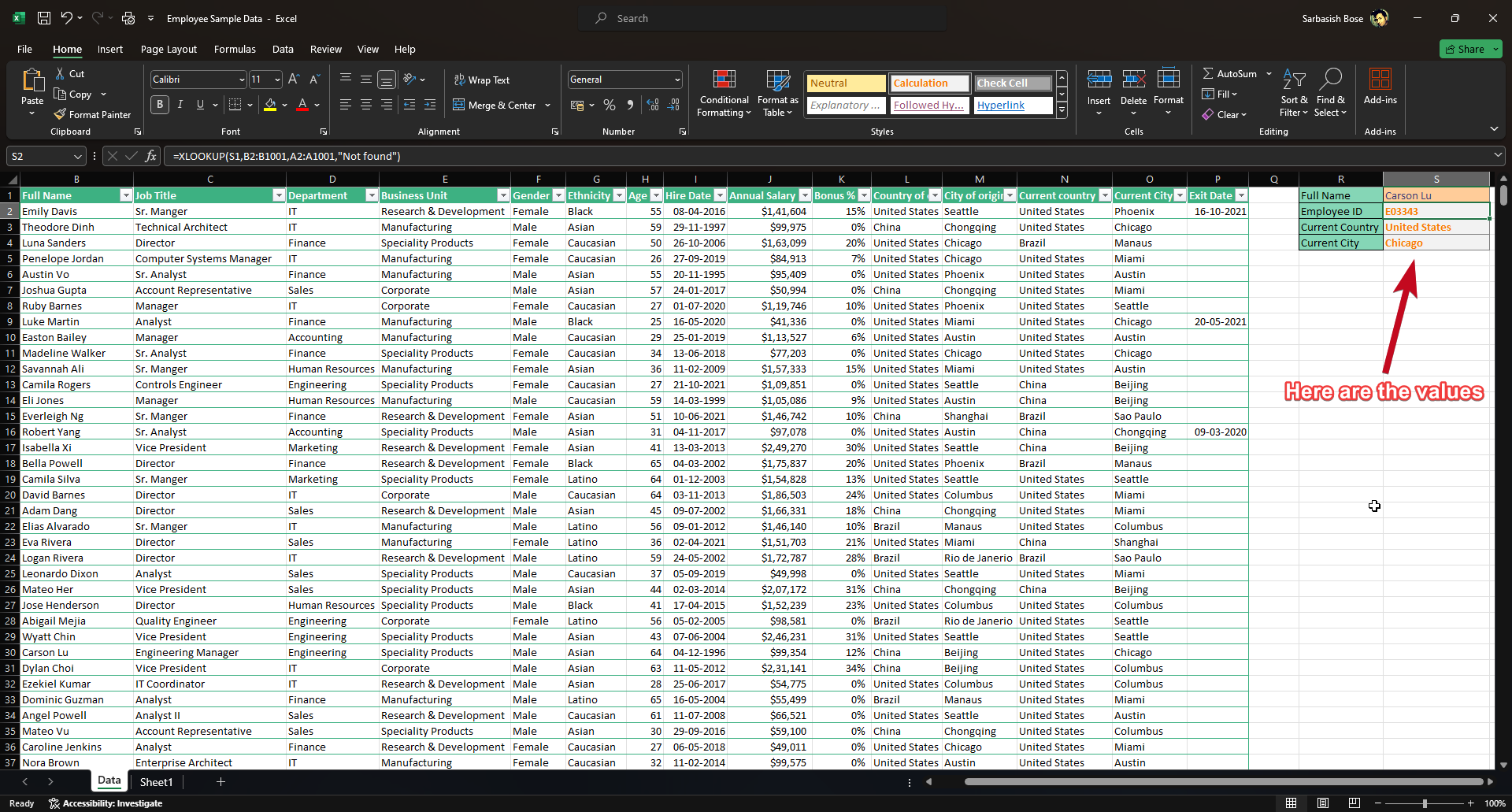
Now, I want to use XLOOKUP to fetch the Employee ID, current country name, and city based on the employee name.
Even though VLOOKUP can be used in this case, there will be limitations, which I will discuss later.
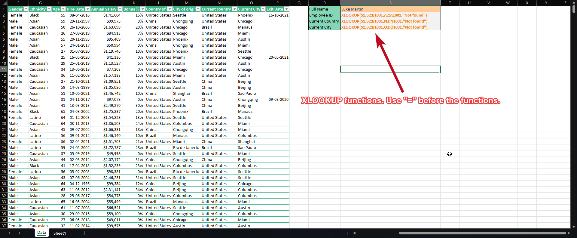
I will enter the name in cell S1, and the corresponding employed ID, country, and city name will automatically be fetched in cells S2, S3, and S4.
So, the entry in the cells S2, S3, and S4 will go as follows:
In U2
=XLOOKUP(S1,B2:B1001,A2:A1001,"Not found")
In U3
=XLOOKUP(S1,B2:B1001,N2:N1001,"Not found")
In U4
=XLOOKUP(S1,B2:B1001,O2:O1001,"Not found")

I have removed the “=” sign in the screenshot for your understanding. However, you should use the “=” before implementing XLOOKUP, just like all other functions in Excel.
I haven’t used any additional arguments here except the “If_not_found” argument. However, you can use one.

Power of XLOOKUP
That was a basic guide on how to use XLOOKUP. Besides this basic implementation, XLOOKUP is a powerful new Microsoft Excel lookup that brings multiple functions under one umbrella. Let’s have a look at why it is so powerful and its dominance over VLOOKUP or HLOOKUP.
- If the search value is not found, you can set an error message to be displayed using XLOOKUP, unlike VLOOKUP or HLOOKUP, where IFERROR needs to be nested in the function to display an error message.
- Depending on how you want to look up in Excel, you either have to use VLOOKUP or HLOOKUP. However, using XLOOKUP, you can search both vertically and horizontally, as you simply need to address the arrays where the values need to be searched and returned.
- VLOOKUP can search only on the right of where the value is found. However, in the case of XLOOKUP, you can search both left and right as you are just addressing the arrays.
- If a new column or row is inserted in the sheet, unlike VLOOKUP or HLOOKUP, it will not alter the results of XLOOKUP, even if the arrays are shifted due to the action.
The XLOOKUP function is a relatively new function on Microsoft Excel, introduced in Excel 2019. So, that’s all about the basics of the XLOOKUP tool in Microsoft Excel. Do you have any questions? Feel free to comment below.

Related Posts
How to Archive a WhatsApp Conversation Without Deleting
How to Clear or Delete Archived Emails in Gmail
How to Clear Google Search History?
2 best Android Apps to open zip or archive files on the smartphone
How to use the XLOOKUP function in Microsoft Excel with Example
How to set up an out-of-office responder on Gmail? Step-by-step guide on setting up a Vacation responder