How to calculate a loan EMI on Google Sheets, Microsoft Excel and other spreadsheet program

We often need loans for personal or business requirements, to start a new business, study abroad, and several other purposes. While credit is an important part of the development of all kinds, it also helps credit institutions like banks to earn profits, and hence offer interest to account holders to help in the overall growth of the economy. But, if you want to get a loan of any kind, it is important to plan your EMIs so that you do not default on the payments and severely impact your credit score. 

While you will be informed about the EMI amount at the time of taking the loan, by the institution like a bank or any other financial institution, I will talk about how you can calculate the EMI for a loan, right on your spreadsheet program like Google Sheets or Microsoft Excel as long as you know the interest rate and the loan tenure. That way you can apply for the loan only after you are ready to pay the EMIs, instead of negotiating with the financial institution at the time of taking the loan.

So, without any further delay, let’s get started with how you can calculate loan EMI using Google Sheets, Microsoft Excel, or any other spreadsheet program.

Formula to calculate loan EMI on a spreadsheet

To calculate the EMI for a loan, there are three things that you will need. The principal amount, i.e. amount that you are borrowing, the interest rate, which is self-explanatory, and the tenure, i.e. number of months that you will need to repay the loan completely. The loan tenure in months is also equal to the number of EMIs that you will pay.

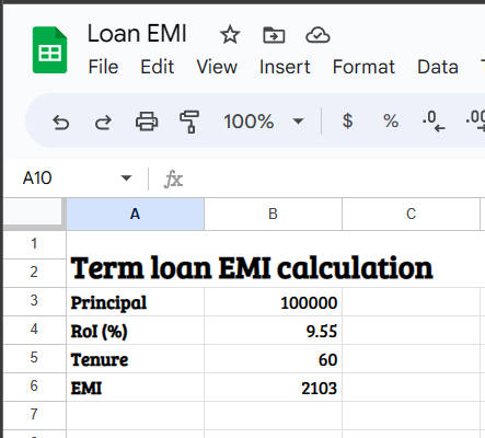
So, you just need a spreadsheet on your preferred platform, and enter these values in different cells as shown in the screenshot below.

We have the principal amount in cell B3, the interest rate in cell B4, and the tenure in months, which is also equal to the number of EMIs in B5, and we want the output or the monthly EMI in cell B6.

So, the formula in cell B6 will go as follows.

=ROUND(((B3*(B4/100/12)*(1+(B4/100/12))^B5)/((1+(B4/100/12))^B5-1)),2)

The result that you will get here will be almost equal to the actual EMI that you will have to pay. Based on the institution that you are borrowing from, the actual EMI can deviate by a small amount, if there are some additional charges.

However, if the cells containing the principal amount and the EMI are formatted for currency, you can ignore the ‘ROUND’ function as the result will be accurate to two decimal places automatically. So, here’s what the formula should look like without the ‘ROUND’ function.

=((B3*(B4/100/12)*(1+(B4/100/12))^B5)/((1+(B4/100/12))^B5-1))

The formula that I have discussed here applies exclusively to term loans. A term loan is a type of loan, where the whole amount is disbursed in one time (except for home loans, and specific loans where it is disbursed in multiple stages), and you repay the loan through EMIs across the loan tenure. However, if you have a demand loan like an overdraft, the interest is calculated daily only on the amount borrowed, where there is no specific tenure, and the calculation displayed here won’t be useful.

So, that was all about how to calculate a loan EMI on Google Sheets and Microsoft Excel. Do you have any questions? Feel free to comment on the same below.